Breadth-First Search
Breadth-first search helps us traverse a graph and search for a given node or vertex; we use the terms vertex and node interchangeably. The underlying logic for this algorithm is simple. It starts with a node (let us call it, source node) and then keeps traversing to its neighbor nodes, one at a time. And once it has traveled to all of its neighbors, it then visits neighbors of the current neighbors. Thus, at each step, it expands outwards from the source node. We will see later on that two of the graph-based algorithms: Dijkstra's algorithm and Prim's algorithm are based on breadth-first search.
Breadth-first search takes the help of a Queue data-structure. It also relies on the ability to mark the nodes: unvisited (color white), visit in progress (gray), and visit done (black). It starts by marking all nodes unvisited. Starting at the source node, it first adds all of its neighbors in the queue -- when adding to the queue, it marks them gray. Going forward the queue forms the basis of the execution. In the next step, it dequeues the first element from the queue and looks at the neighbors of this element. If a neighbor is white, then it adds it to the queue. Else, it ignores it since it has either been visited or is being visited. Breadth-first search assumes that the nodes in the graph are connected. If they are not, then the algorithm traverses only those nodes that belong to the partition of the source node.
Let us now see how the Breadth-first search algorithm works in more detail. For that, let us start with a simple graph (provided below). The graph has 5 vertices and 5 edges. For the sake of simplicity, we keep the graph undirected.
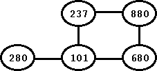
Figure: An Undirected Graph
The first thing we do is to mark all vertices as white. As Step 1, we start with the source vertex (let us say, node 101) and add this node to the queue. Hence, at the first step, the only vertex in the queue would be the node 101. We mark this node gray since we are still working on it and have not added its neighbors yet. Next, we dequeue the next value from the queue (in this case, 101) and add all of its neighbor vertices to the queue. With that, the queue now has 680, 237, and 280. When doing so, we mark all of these vertices as gray since they are being processed. Once all the neighbors are added, we are done with vertex 101 and so, we mark it black. We continue with the remaining steps. Dequeue the node from the queue, add its neighbor vertex nodes, if they are not already added, and mark the current node black. We do this till we have no more elements left in the queue. Once we reach the last step, all the nodes in the graph would be black. And that would complete the breadth-first search.
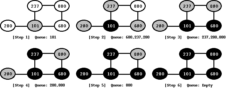
Figure: Breadth-First Search
The above steps provide insight into breadth-first search algorithm. As we discussed earlier, every step adds neighboring nodes. Only when we are done with all the neighbors, we go ahead and add the next layer of neighbors. Thus, when we start to add neighbors of node 101, we first add all of its immediate neighbors (680, 237, and 280) and only once we are done with that, we begin to add the next set of neighbors -- in this case, node 880.
Implementation
For our implementation of a breadth-first-search, we take help of two data-structures. The first one is an Adjacency List. The second one is a Queue. We have provided both of these data-structures in our Data-Structure module. The reason why we reuse these two existing implementations is that without doing that we would end up implementing both adjacency list and queue in the implementation. And that would add many more lines of code to our implementation making it less readable. We recommend the reader to go through these data-structures first.
Our implementation of Adjacency List and Queue are provided in terms of both header file and an implementation file. For our implementation on this page, we simply add the header files ("adjacency_list.h" and "queue.h") so that we can access their APIs. In terms of APIs, we use the following APIs from adjacency list: adjlist_add_vertex() to add a vertex to the adjacency list, adjlist_add_edge() to add an edge to the adjacency list, adjlist_free() to free the adjacency list, and adjlist_print() to print adjacency list. For queue, we use the following APIs: queue_init() to initialize the queue, queue_enqueue() to add vertices to the queue, and queue_dequeue() to pop the next vertex from the queue.
With that, let us provide the implementation of a simple breadth-first search. The implementation takes the root of the graph as the source node. Since the graph is connected, even if we were to choose some other vertex, we would still traverse all the nodes.
 #include "stdio.h"
 #include "stdbool.h"
 #include "queue.h"
 #include "adjacency_list.h"

 vertex_node *graph_root = NULL; /* Root of the graph */

 void bfs_print_queue (queue *sq) {
     queue_elem *elem = NULL;

     printf("Printing Queue (size: %d): ", queue_get_size(sq));
     for (elem = sq->head; elem != NULL; elem = elem->next) {
         printf("%d  ", *(int *)(elem->data));
     }
     printf("\n");
 }

 void bfs_run (vertex_node *source_node) {
     vertex_node *vnode = NULL, *internal_vnode = NULL;
     edge_node *enode = NULL;
     queue q;
     int err;

     /* Initialize the queue */
     queue_init(&q);

     /* First, color all the vertices white. */
     for (vnode = source_node; vnode != NULL; vnode = vnode->next_vnode) {
         vnode->color = COLOR_WHITE;
     }

     vnode = source_node;
     vnode->color = COLOR_GRAY;
     queue_enqueue(&q, vnode);
     while (true) {
         bfs_print_queue(&q);
         adjlist_print(graph_root);
         vnode = (vertex_node *)queue_dequeue(&q, &err);
         if (!vnode) {
             printf("\n[%s] BFS Done\n", __FUNCTION__);
             return;
         }
         /* Run through all the edges for this node. */
         printf("\n[%s] BFS: current Vertex: %d \n", __FUNCTION__, vnode->val);
         for (enode = vnode->list_enode; enode != NULL; enode = enode->next_enode) {
             internal_vnode = (vertex_node *)enode->parent_vnode;
             if (internal_vnode->color == COLOR_WHITE) {
                 internal_vnode->color = COLOR_GRAY;
                 queue_enqueue(&q, internal_vnode);
             }
         }
         /* This node is done. */
         vnode->color = COLOR_BLACK;
     }
 }

 int main () {
     int vertices[] = {101, 237, 680, 280, 880};
     int edges[][2] = {{101, 680}, {101, 237}, {880, 680}, {101, 280}, {237, 880}};
     int len_vertices, len_edges, i;

     /* Add the vertices. */
     len_vertices = sizeof(vertices)/sizeof(vertices[0]);
     for (i = 0; i < len_vertices; i++) {
         adjlist_add_vertex(&graph_root, vertices[i], NULL);
     }

     /* Add the edges. */
     len_edges = sizeof(edges)/sizeof(edges[0]);
     for (i = 0; i < len_edges; i++) {
         adjlist_add_edge(graph_root, edges[i][0], edges[i][1], 0);
     }

     /* Run BFS on this */
     bfs_run(graph_root);

     /* Done with the Adjacency List. Free it */
     adjlist_free(&graph_root);
 }
The above implementation starts with the main() function, where we first build the adjacency list for the graph. We build the graph using input from two arrays: vertices and edges. We add vertices from the vertex array using adjlist_add_vertex(). We add edges from the edges array using adjlist_add_edges(); when adding the edges, we keep the edge weight as 0, since we are using a non-weighted graph. Once the graph is ready, we pass the root of the graph as the source node and run the bfs_run() function.
The bfs_run() function starts with the source vertex. Next, it adds all of its edges to the queue. Once that is done, it enters the while loop. At each iteration of the loop, it dequeues the next vertex node from the queue, prints the node, and then proceeds to enqueue all the nodes of the newly selected vertex node. When enqueuing, we make sure to add only those vertices that are white in color since if it is black or gray, then it means that either its processing is done or is in progress. Also, when we enqueue a node that is white, we mark it gray so that we know that it is being processed. Once we print the newly selected vertex, then we mark it as black since we are done with this node. Next, we dequeue the next vertex node from the queue and the loop continues. Once bfs_run() is done, the main() function calls adjlist_free() to free up the resources malloced when building the adjacency list.
To show the progress of the algorithm, the implementation also uses adjlist_print() to print the adjacency list from time to time -- we do this to show the color-variation of individual node as the algorithm progresses. In addition, the implementation also uses bfs_print_queue() to print the elements in the queue.
In terms of time-complexity, the above algorithm is linear with respect to the the edges and vertices. In terms of vertices, we visit each vertex once. If we hit the same vertex again, then we simply ignore it since it has already been added to the queue. Thus, the running time with respect to vertices is O(V). In terms of edges, we visit an edge of a graph when we process its two parent vertices after they gets dequeued. So, all edges are visited twice. Thus, the running time with respect to edges is O(E). In other words, the total time complexity as O(V+E).
At this point, we are ready to fire the program! For that, we pass the above file (let us call it "bfs.c") along with the implementation of the adjacency list (let us say, "adjacency_list.c") and queue (let us say, "queue.c") to the GCC compiler. The output (provided below) confirms that queue starts with 101 and then keeps expanding by visiting the next set of neighbors. Further, the output shows that the color of the vertices go from white (value = 1), to gray (value = 2), and finally to black (value = 3).
 user@codingbison $ gcc bfs.c adjacency_list.c  queue.c -o bfs
 user@codingbison $ ./bfs
 Printing Queue (size: 1): 101
 [adjlist_print] Print the Adjacency List
         Vertex [101][Color: 2]: -- Edge [680 (0)] -- Edge [237 (0)] -- Edge [280 (0)]
         Vertex [237][Color: 1]: -- Edge [101 (0)] -- Edge [880 (0)]
         Vertex [680][Color: 1]: -- Edge [101 (0)] -- Edge [880 (0)]
         Vertex [280][Color: 1]: -- Edge [101 (0)]
         Vertex [880][Color: 1]: -- Edge [680 (0)] -- Edge [237 (0)]

 [bfs_run] BFS: current Vertex: 101
 Printing Queue (size: 3): 680  237  280
 [adjlist_print] Print the Adjacency List
         Vertex [101][Color: 3]: -- Edge [680 (0)] -- Edge [237 (0)] -- Edge [280 (0)]
         Vertex [237][Color: 2]: -- Edge [101 (0)] -- Edge [880 (0)]
         Vertex [680][Color: 2]: -- Edge [101 (0)] -- Edge [880 (0)]
         Vertex [280][Color: 2]: -- Edge [101 (0)]
         Vertex [880][Color: 1]: -- Edge [680 (0)] -- Edge [237 (0)]

 [bfs_run] BFS: current Vertex: 680
 Printing Queue (size: 3): 237  280  880
 [adjlist_print] Print the Adjacency List
         Vertex [101][Color: 3]: -- Edge [680 (0)] -- Edge [237 (0)] -- Edge [280 (0)]
         Vertex [237][Color: 2]: -- Edge [101 (0)] -- Edge [880 (0)]
         Vertex [680][Color: 3]: -- Edge [101 (0)] -- Edge [880 (0)]
         Vertex [280][Color: 2]: -- Edge [101 (0)]
         Vertex [880][Color: 2]: -- Edge [680 (0)] -- Edge [237 (0)]

 [bfs_run] BFS: current Vertex: 237
 Printing Queue (size: 2): 280  880
 [adjlist_print] Print the Adjacency List
         Vertex [101][Color: 3]: -- Edge [680 (0)] -- Edge [237 (0)] -- Edge [280 (0)]
         Vertex [237][Color: 3]: -- Edge [101 (0)] -- Edge [880 (0)]
         Vertex [680][Color: 3]: -- Edge [101 (0)] -- Edge [880 (0)]
         Vertex [280][Color: 2]: -- Edge [101 (0)]
         Vertex [880][Color: 2]: -- Edge [680 (0)] -- Edge [237 (0)]

 [bfs_run] BFS: current Vertex: 280
 Printing Queue (size: 1): 880
 [adjlist_print] Print the Adjacency List
         Vertex [101][Color: 3]: -- Edge [680 (0)] -- Edge [237 (0)] -- Edge [280 (0)]
         Vertex [237][Color: 3]: -- Edge [101 (0)] -- Edge [880 (0)]
         Vertex [680][Color: 3]: -- Edge [101 (0)] -- Edge [880 (0)]
         Vertex [280][Color: 3]: -- Edge [101 (0)]
         Vertex [880][Color: 2]: -- Edge [680 (0)] -- Edge [237 (0)]

 [bfs_run] BFS: current Vertex: 880
 Printing Queue (size: 0):
 [adjlist_print] Print the Adjacency List
         Vertex [101][Color: 3]: -- Edge [680 (0)] -- Edge [237 (0)] -- Edge [280 (0)]
         Vertex [237][Color: 3]: -- Edge [101 (0)] -- Edge [880 (0)]
         Vertex [680][Color: 3]: -- Edge [101 (0)] -- Edge [880 (0)]
         Vertex [280][Color: 3]: -- Edge [101 (0)]
         Vertex [880][Color: 3]: -- Edge [680 (0)] -- Edge [237 (0)]

 [bfs_run] BFS Done